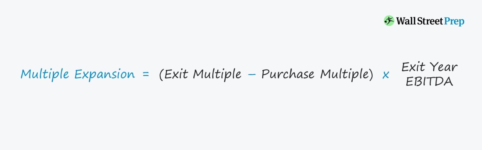
Multiple Expansion is when an asset is purchased and later sold at a higher valuation multiple relative to the original multiple paid.
If a company undergoes a leveraged buyout (LBO) and is sold for a higher price than the initial purchase price, the investment will be more profitable to the private equity firm.
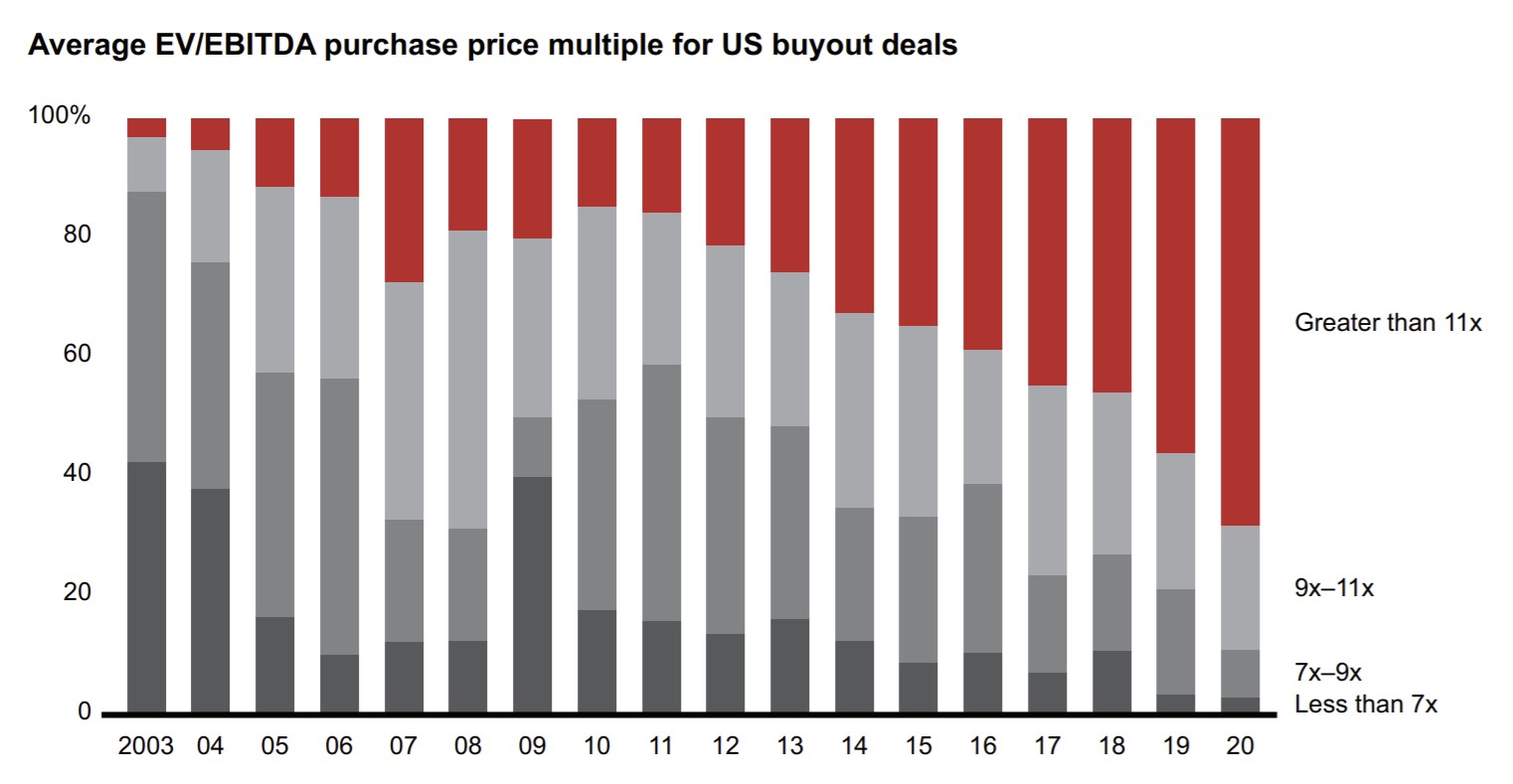
When it comes to leveraged buyouts (LBOs), pricing is arguably the most important consideration.
Simply put, the objective behind multiple expansion is to “buy low, sell high”.
Once a financial sponsor acquires a company, the firm seeks to gradually pursue growth opportunities while identifying operational inefficiencies where improvements could be made.
Some common examples of potential value-add opportunities are:
Reducing Employee Headcount
Closing Redundant Facilities
Eliminating Unnecessary Functions
Divesting Non-Core Assets
Negotiating Longer-Term Customer Contracts
Geographic Expansion
If the changes implemented are successful, the post-LBO company will have higher profit margins and higher-quality revenue (i.e. recurring, stable), which is essential in the context of leveraged buyouts (LBOs) due to the highly levered capital structure.
While not a guarantee by any means, the odds of exiting at a higher multiple improves if the private equity firm is able to implement strategic adjustments such as the ones mentioned above.
The inverse of multiple expansion is called multiple contraction, which means the investment was sold for a lower multiple than the original acquisition multiple. In such cases, the buyer likely overpaid and subsequently took a loss when selling the company.
However, for larger-sized LBOs, minor multiple contraction can be acceptable (and often be expected). This is because the number of potential buyers is reduced as fewer buyers can afford to purchase the asset.
LBO Purchase Multiple and Exit Multiple Assumptions
In practice, the majority of LBO models use the conservative assumption of exiting at the same multiple as the entry multiple.
Given the amount of uncertainty regarding the market conditions and unforeseeable events that could have a significant impact on the exit multiple, the recommended industry best practice is to set the exit multiple assumption equal to the purchase multiple.
Even if the private equity firm expects to take actions during its ownership period that could increase the exit multiple (and returns), the most important takeaway is that the private equity firm's thesis and expected returns should not be overly reliant on selling at a higher valuation.
Multiple expansion can frequently be caused by favorable secular trends and market timing (e.g. COVID-19 and telemedicine).
For instance, let’s say that a financial sponsor acquires a company for 7.0x EBITDA. If the target company’s last twelve months (LTM) EBITDA is $10mm as of the purchase date, then the purchase enterprise value is $70mm.
If the financial sponsor later sells the same company for 10.0x EBITDA, then the net positive difference between the 7.0x and 10.0x is the concept of multiple expansion.
Even if the company's EBITDA remains unchanged at $10mm, if the sponsor exits the investment five years later but at a 10.0x exit multiple, $30mm of value would have been created – all else being equal.
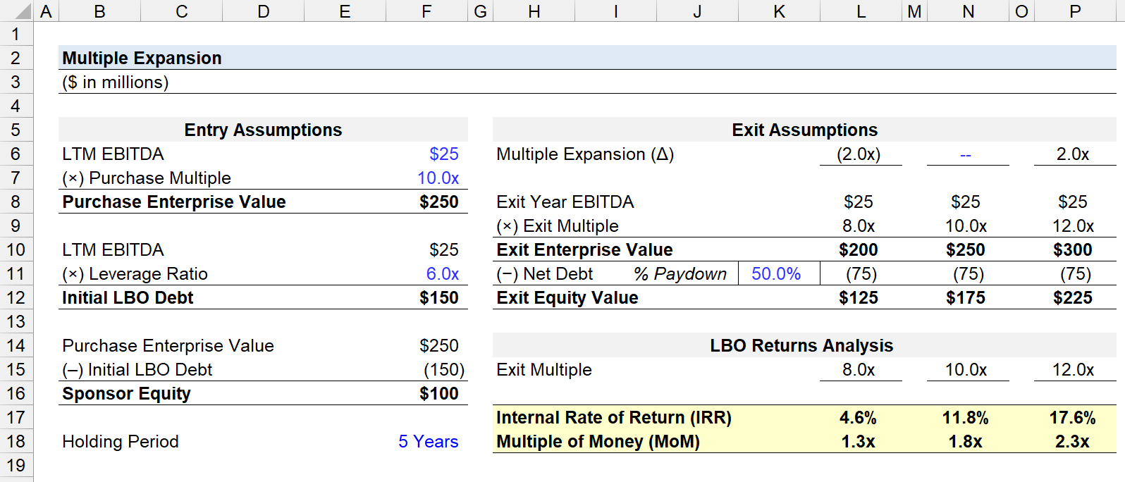
First, the entry assumptions we’ll be using are as follows:
LTM EBITDA = $25mm
Purchase Multiple = 10.0x
In our hypothetical transaction, the LBO target has generated $25mm in LTM EBITDA, which is the metric upon which the purchase multiple will be applied.
By multiplying our LTM EBITDA by the purchase multiple, we can calculate the purchase enterprise value – i.e. the total purchase price paid to acquire the company.
Next, we must figure out the initial investment contributed by the financial sponsor, or the private equity firm.
Here, we’re assuming that the total leverage ratio was 6.0x LTM EBITDA and there are no other providers of capital other than the single leverage provider (i.e. debt-holder) and the financial sponsor. Since the purchase multiple was 10.0x, we can deduce the sponsor equity contribution was 4.0x LTM EBITDA (i.e. four turns of EBITDA).
We can then multiply the LTM EBITDA by the sponsor equity contribution multiple to figure out how much the financial sponsor had to pay for the deal to close.
Sponsor Equity = 4.0x × $25mm = $100mm
Before we move onto the exit multiples section, there are two more assumptions for our exercise:
Holding Period = 5 Years
Cumulative Debt Paydown = 50%
In the five-year holding period during which the acquired LBO target belongs to the sponsor, half of its total debt financing is expected to be paid down.
On the date of exit, there should be $75mm in debt remaining on the balance sheet of the company.
2. LBO Exit Assumptions
Since our entry assumptions have all been set up, we’re ready to see the impact of the exit multiple on the returns of an LBO.
We’ll be comparing three scenarios with different exit multiples:
8.0x: Multiple Contraction of – 2.0x
10.0x: Purchase Multiple = Exit Multiple
12.0x: Multiple Expansion of 2.0x
To isolate the impact of the exit multiple as much as possible, the LTM EBITDA assumed at exit is going to be the same as the LTM EBITDA on the date of purchase – i.e. no EBITDA growth is assumed throughout the holding period.
Given the unchanged exit $25mm LTM EBITDA, we apply the corresponding exit multiple against this figure.
For each case, we must subtract the $75mm in debt. Note that for simplicity, we are assuming there is no cash remaining on the B/S at exit – thus net debt is equal to total debt.
From the exercise we just completed, we can see the extent of how sensitive the returns on n LBO investment are to the purchase multiple and exit multiple.







No comments yet.