PV Function

How to Use PV Function in Excel

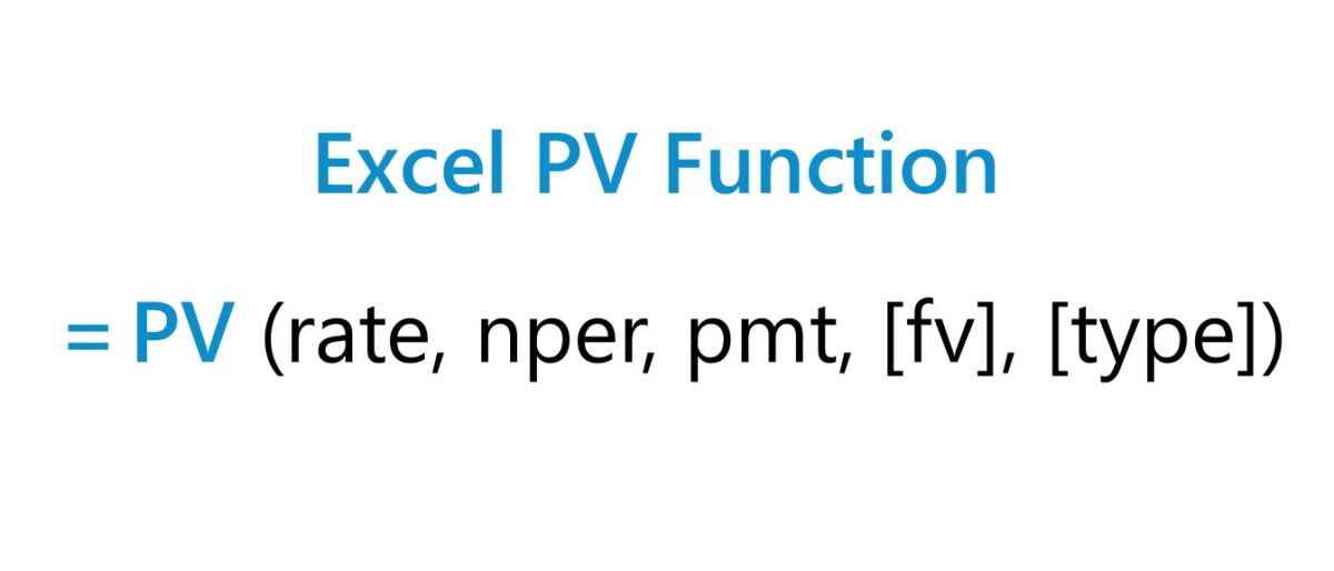
The PV function is a built-in feature in Excel used to determine the present value of a series of future cash flows, i.e. an annuity.

The present value (PV) is a fundamental concept in finance based on the “time value of money”, which states that a dollar received today is worth more than a dollar received in the future.

Therefore, the future cash flows of an investment—whether it consists of interest payments on a loan or amortization of the original principal—must be discounted back to the current date to reflect the TVM principle.

The Excel “PV” function can only be used if the stream of cash flows remain constant (and the interest rate is fixed). Otherwise, the “NPV” function would be more appropriate given irregular cash flows.

PV Function Formula Syntax

The formula to use the PV function in Excel is as follows.

• “rate” → Interest Rate (%)
• “nper” → Number of Compounding Periods
• “pmt” → Periodic Payment
• “fv” → Future Value
• “type” → Type of Payment (0 = Payment at End of Period; 1 = Payment at Beginning of Period)

The latter two arguments—the “fv” and “type”—are enclosed in brackets to denote that those are optional inputs.

1. Future Value → If the “fv” argument is omitted (i.e. left blank), the assumption is that the value of the investment on the date of the final payment is zero.
2. Type of Payment → If the “type” argument is omitted, the default assumption by Excel is that the payments are received at the end of each period.

The “pmt” argument can be omitted too, based on the condition that there is a value entered for the “fv” argument. Otherwise, the “pmt” argument is required.

Periodicity Conversion Chart (“rate” and “nper”)

The interest rate (”rate”) and number of compounding periods (”nper”) must be adjusted for consistency in terms of timing.

Excel PV Function: Annuity vs. Perpetuity Calculation

• Annuity → The PV function pertains to an annuity, which is a fixed stream of periodic payments (i.e. cash flows) with a stated maturity date at which the payments stop.
• Perpetuity → In contrast, a perpetuity is a constant stream of fixed payments that continue indefinitely.

The formula in Excel to calculate the present value (PV) of a perpetuity is as follows.

PV Function Calculator – Excel Template

We’ll now move on to a modeling exercise, which you can access by filling out the form below.

You’re logged in! Form submission not required. Access your file below.

Download File

1. Present Value (PV) of Bond Assumptions

Suppose you’re tasked with calculating the present value (PV) of a semi-annual corporate bond with a face value (FV) of $100,000 and ten-year maturity.

Furthermore, the annual coupon rate is 6.0% and the coupon is paid at the end of each period.

The annual market rate—i.e. the interest rate derived from comparable bonds belonging to issuers with similar credit ratings—is 8.0%.

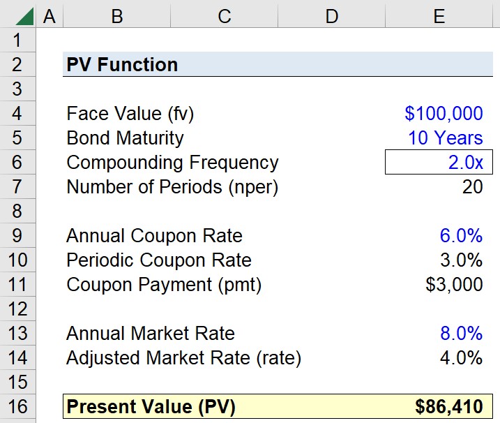
The stated assumptions so far are summarized here:

• Face Value (FV) = $100,000
• Bond Maturity = 10 Years
• Compounding Frequency = 2.0x (Semi-Annual Bond)
• Annual Coupon Rate = 6.0%
• Annual Market Rate = 8.0%

2. “nper”, “pmt” and “rate” Calculation Example

To reiterate from earlier, we must first ensure the periodicity of each input is consistent.

Since the bond maturity, the coupon payment, and the market rate are all expressed on an annual basis, we must convert them to a semi-annual basis.

• Number of Periods (nper) = 10 Years × 2 = 20
• Periodic Coupon Rate = 6.0% ÷ 2 = 3.0%
• Adjusted Market Rate = 8.0% ÷ 2 = 4.0%

The only input remaining that we must compute is the periodic coupon payment, which we’ll calculate by multiplying the periodic coupon rate by the face value (FV) of the bond.

• Coupon Payment (pmt) = 3.0% × $100,000 = $3,000

3. Excel PV Function Calculation Example

We now have all the required inputs, so the final step is to enter them into the Excel PV function formula:

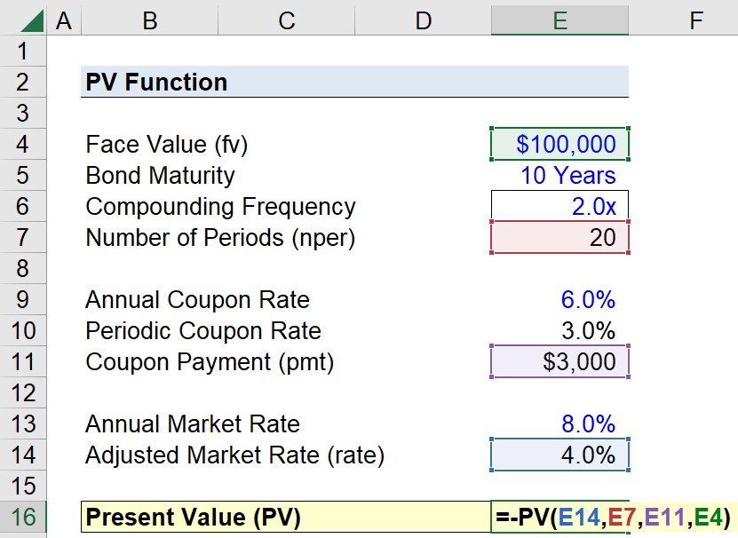
The “type” argument is left blank, since earlier we said that the bond payments occur at the end of each period, which is the default setting.

We’ve also entered a negative sign in front of our equation as an optional step. Intuitively, it would make sense for the present value to be a negative value given that it is a cash outflow, depending on the perspective.

In closing, the present value of the bond in our hypothetical scenario comes out to $86,410.

Turbo-charge your time in Excel

Used at top investment banks, Wall Street Prep’s Excel Crash Course will turn you into an advanced Power User and set you apart from your peers.

Learn More