What is the Excel SUMIF Function?
The SUMIF Function in Excel returns the sum of the values in a selected range that meet a specified criterion.

The SUMIF Function in Excel returns the sum of the values in a selected range that meet a specified criterion.
The SUMIF function is a built-in feature of Excel utilized to calculate the sum of values in a range based on a “TRUE” or “FALSE” condition.
The specified criteria can be a logical condition using numeric values, as well as dates and text, where the calculation only includes the value of the cells within the selected range that meet the given condition.
For instance, a practical use-case of the SUMIF function would be to calculate the sum of the sales generated by a specific employee, which enables the company’s upper management to evaluate the sales efficiency of each individual on the sales team.
The SUMIF function, however, is constrained to one condition. If the task at hand requires a criterion with multiple conditions, then the SUMIFS function would be more appropriate.
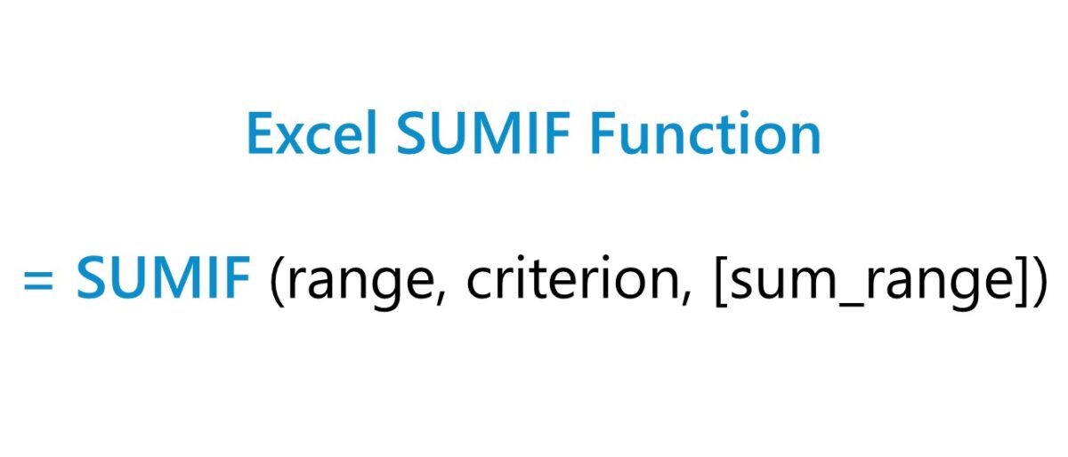
The Excel SUMIF function formula is as follows.
The brackets around “sum_range” indicate it is optional and can be omitted, i.e. left blank. If omitted, the default setting is to calculate the sum using the range selected in the condition.
The criterion of the SUMIF function can support logical operators and wildcards.
In order for the function to work as intended, the proper syntax must be used.
While there are exceptions, such as purely numeric (e.g. =10) or binary conditions (e.g. True, False), operators must be enclosed in double quotes ("").
Any criterion with a cell reference must have the operator enclosed in parentheses and concatenated (e.g. “>"&A1)
The most common logical operators are as follows.
| Criterion | Description | Example |
|---|---|---|
| = |
|
|
| <> |
|
|
| > |
|
|
| < |
|
|
| >= |
|
|
| <= |
|
|
| “” |
|
|
| “<>” |
|
|
For the SUMIF functions containing wildcard characters:
| Wildcards | Description |
|---|---|
| Question Mark (?) |
|
| Asterisk (*) |
|
| Tilde (~) |
|
We’ll now move on to a modeling exercise, which you can access by filling out the form below.


Suppose we’re tasked with evaluating a company’s revenue segmentation based on its latest fiscal year.
The company's $8 million in revenue came from ten customers, which are categorized on the basis of either a “Large Enterprise” or “SME”.
The data set below contains the revenue per customer and each categorization.
| Customer | Category | Revenue |
|---|---|---|
| A | Large Enterprise | $1,000,000 |
| B | SME | 400,000 |
| C | SME | 120,000 |
| D | Large Enterprise | 1,100,000 |
| E | Large Enterprise | 1,400,000 |
| F | SME | 280,000 |
| G | Large Enterprise | 1,800,000 |
| H | SME | 240,000 |
| I | SME | 160,000 |
| J | Large Enterprise | 1,500,000 |
| Total Revenue | $8,000,000 |
We’ll determine the breakdown of revenue by customer category using the SUMIF function.
Starting with the large enterprise customer category, the following Excel equation determines the revenue from customers that fall under just that categorization.
The range highlights the "Category" column to identify which customers meet the customer type criterion.
Once the customers to include in the calculation are determined, the revenue amounts corresponding to the customers that meet the criterion are calculated for the sum.
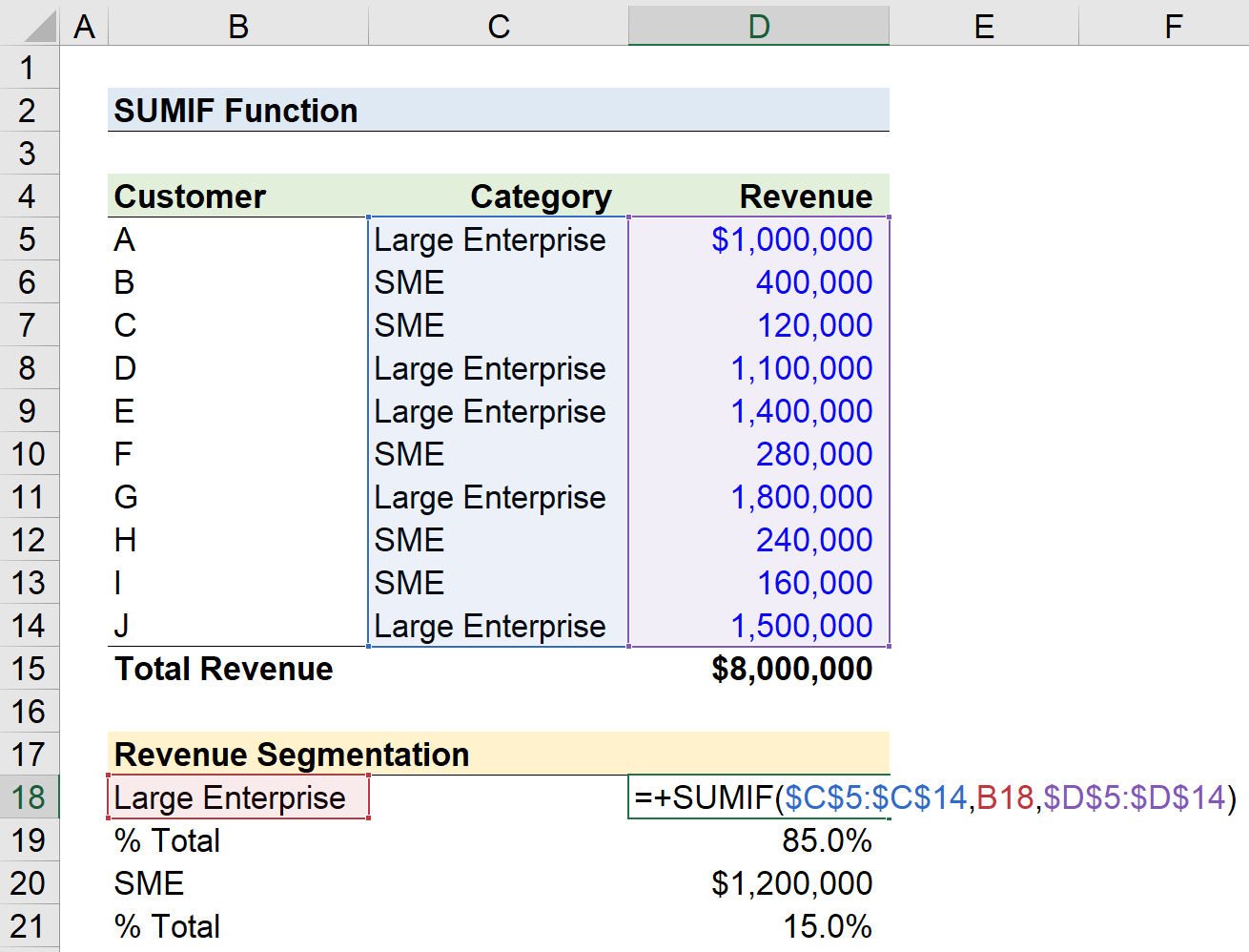
The revenue attributable to large enterprise customers was $6.8 million (and 85.0% of the total revenue).
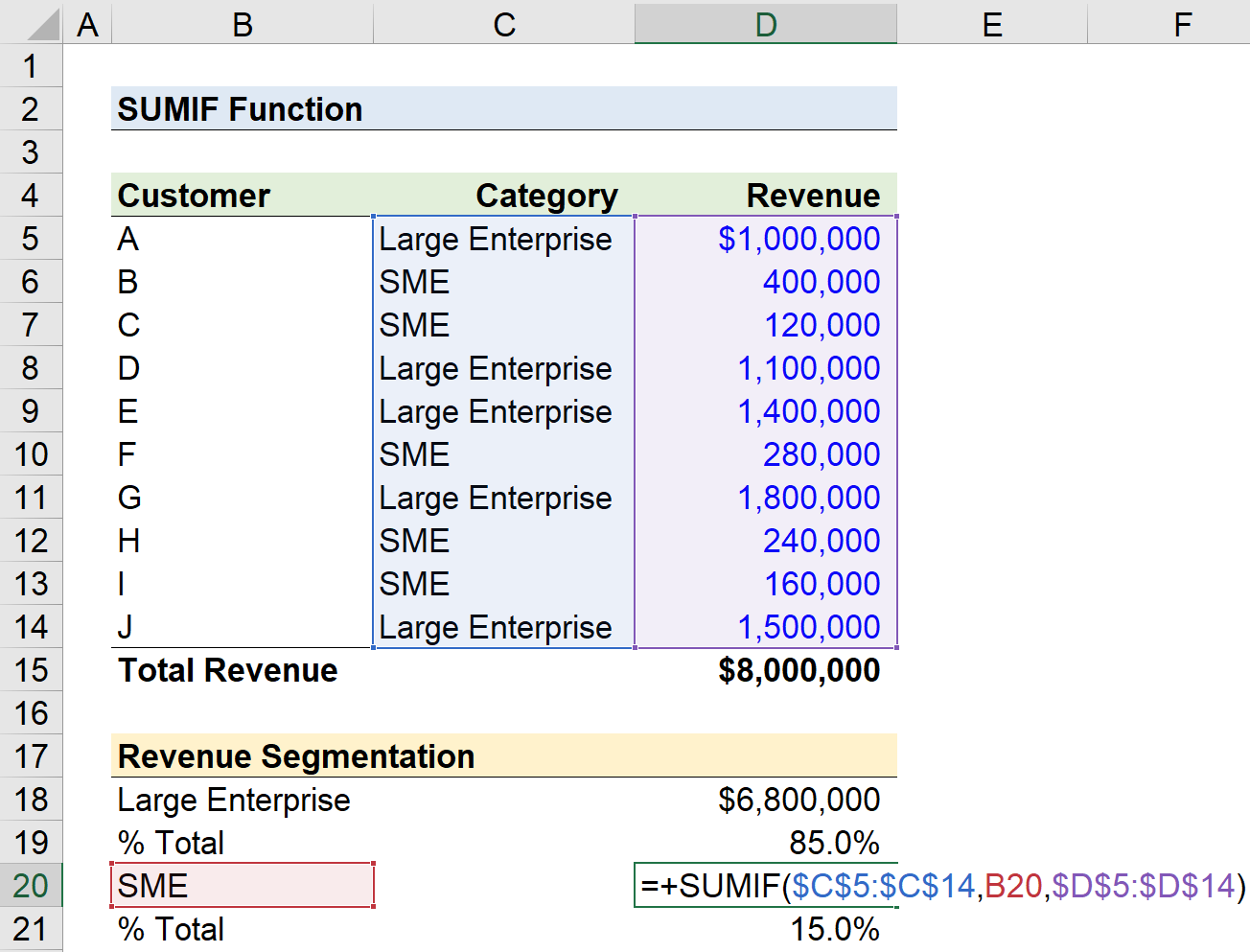
In the next step, we’ll repeat the process, but now for the SME customer category.
Since we anchored the cells (F4) in the prior step, the only adjustment necessary is the criterion.
SME customers contributed the remaining $1.2 million (and 15.0% of the total revenue).
In the next part of our exercise, let's assume that we're tasked with calculating the sum of revenue based on two separate criteria:
For the first portion, we'll use the following formula to determine the customer revenue that is greater than or equal to $1.2 million.
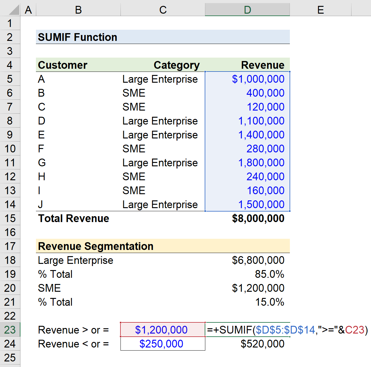
Since our criteria are based on revenue size rather than the customer category, we can omit the "sum_range", since both the criteria and the sum are identified and calculated from the same column.
The total revenue coming from customers that generated at least $1.2 million each comes out to $4.7 million.
In the final part, we'll calculate the sum of the revenue that was less than or equal to $250k.
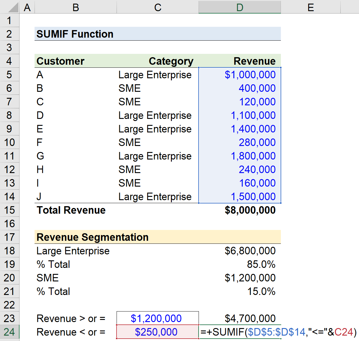
In conclusion, the sum of revenue contributed by customers that generated at most $250k was $520k.




No comments yet.