PPMT Function

How to Use PPMT Function in Excel?

The Excel “PPMT” function calculates the principal payments required to be paid on a loan.

The borrower, as part of the financing arrangement, is contractually obligated to pay interest on a traditional loan and portions of the principal until the entire loan principal is repaid.

For instance, a consumer that takes out a mortgage or auto loan to finance a purchase must make monthly payments to the lender until the principal is repaid in full, while servicing interest expense obligations simultaneously.

But while the interest paid in each period is based on the outstanding principal balance, the interest payments themselves do not reduce the principal.

In the PPMT function, there are two notable assumptions regarding the loan.

1. Fixed Interest Rate → The loan is assumed to have a fixed interest rate (i.e. the rate remains constant and unaffected by a benchmark rate, as in the case of debt securities priced with floating interest rates).
2. Constant Payment Value → The other assumption is that the total payments are constant throughout the term of the borrowing, i.e. akin to installment payments, where the payment dates and amounts due are fixed and predictable.

Real Estate Interview Guide | File Download Form

You’re logged in! Form submission not required. Access your file below.

Download File

Sources of Loan Yield: Interest vs. Principal Payments

The yield earned by a lender on a loan issuance stems primarily from two sources:

1. Periodic Interest Payments → The interest represents income to the lender (i.e. ”inflow of cash”) and the dollar amount charged is a function of the interest rate, which reflects the riskiness of providing capital in the form of debt to the borrower (i.e. credit rating and default risk). Yet, in spite of the constant payment value, the interest and principal payments are not equivalent in every period. Rather, because interest is in part determined by the principal value, a greater proportion of the payment shifts towards the principal payments as more of the principal is paid off over time.
2. Principal Payments → The principal payments, otherwise known as the amortization of the loan, is the gradual reduction in the loan’s outstanding balance. In short, each principal payment reduces credit risk because the capital is returned to the original owner.

The repayment of principal is the return of borrowed capital, so the upside in yield comes from the interest rate (and to reiterate, the value of the interest payments is based on the outstanding principal). However, the capital at risk, i.e. the potential downside, is the loan principal.

Excel PMT vs. PPMT vs. IPMT Function

Two common Excel functions closely related to the “PPMT” function are “PMT” and “IPMT”.

• “=PMT” → The “PMT” function in Excel calculates the periodic payment on a loan, inclusive of both the interest and principal.
• “=IPMT” → In contrast, the “IPMT” in Excel calculates only the interest paid on a loan, as suggested by the “I” in front that stands for "interest.”

The missing piece between the above two functions is the principal payments, which the PPMT function is intended to calculate.

• IPMT Function → Interest
• PPMT Function → Principal
• PMT Function → Principal + Interest

However, it is important to note that there are often other fees and incurred costs such as taxes that can impact the lender’s yield.

Excel PPMT Function Formula

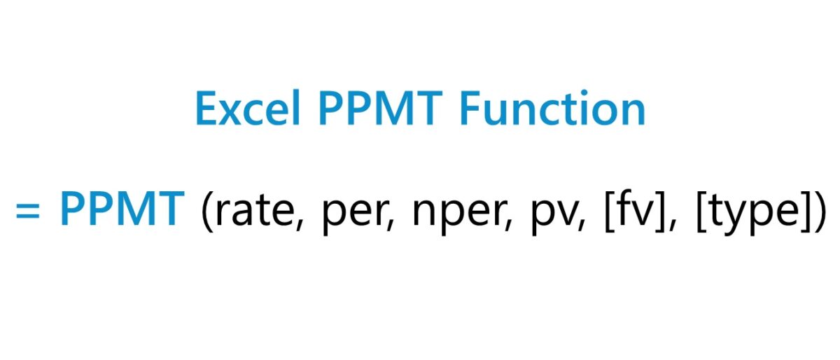
The formula for using the PPMT function in Excel is as follows.

The brackets around “fv” and “type” denote that the two are optional inputs that can be omitted, i.e. left blank.

In terms of the sign convention, the interest and principal payments represent “outflows” of cash to the borrower, so the returned values will be expressed as negative numbers.

The following table can be referenced to confirm the interest rate and number of periods are adjusted properly for the units to be consistent.

For example, imagine a borrower took out an 8-year loan with an annual interest rate of 6.0% paid on a quarterly basis. In this case, the adjusted (i.e. quarterly) interest rate is 1.5%.

• Monthly Interest Rate (rate) = 6.0% ÷ 4 = 1.5%

The number of periods must also be adjusted for the periodicity to match.

The borrowing term in our example was stated in years, so we must multiply it by the payment frequency, i.e. the number of compounding periods, or quarters.

• Number of Periods (nper) = 8 Years × 4 = 32 Periods

PPMT Excel Function Syntax

The table below describes the syntax of the Excel PPMT function in more depth.

PPMT Function Calculator – Excel Template

We’ll now move on to a modeling exercise, which you can access by filling out the form below.

Excel Template

You’re logged in! Form submission not required. Access your file below.

Download File

1. Principal Payment on Loan Exercise Assumptions

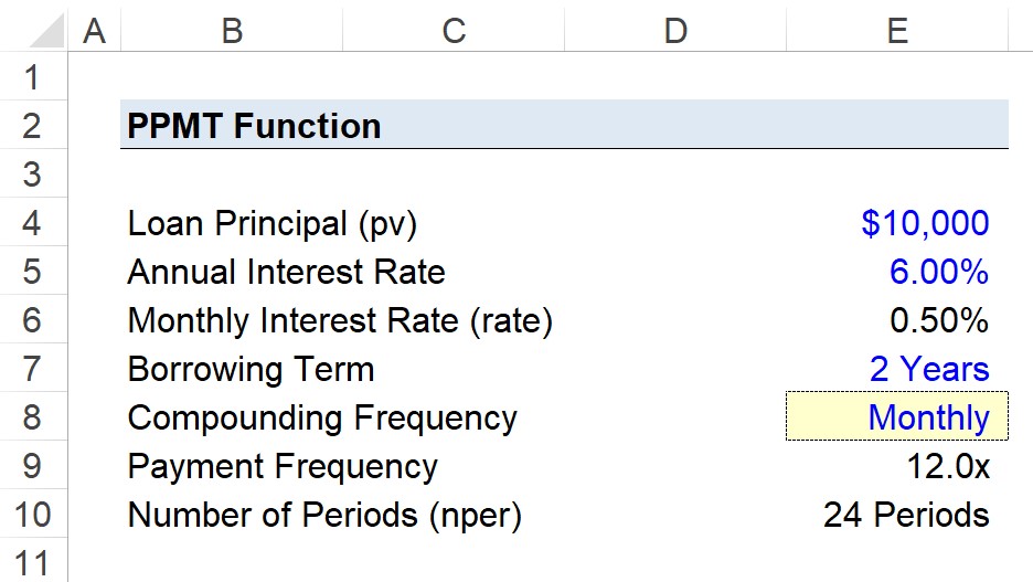
Suppose a consumer has taken out a $10,000 personal loan with a stated annual interest rate of 6.00%, with monthly payments due at the end of each month.

• Loan Principal (pv) = $10,000
• Annual Interest Rate (%) = 6.00%
• Borrowing Term = 2 Years
• Compounding Frequency = Monthly (12x)

The next two steps are to convert our 6.0% annual interest rate into a monthly interest rate, followed by converting our 2-year borrowing term into months.

Using the following equations, we calculate the monthly interest rate as 0.50% and the number of periods as 24 months.

• Monthly Interest Rate (rate) = 6.00% ÷ 12 = 0.50%
• Number of Periods (nper) = 2 Years × 12 = 24 Periods

2. Payment Frequency and “nper” Calculation

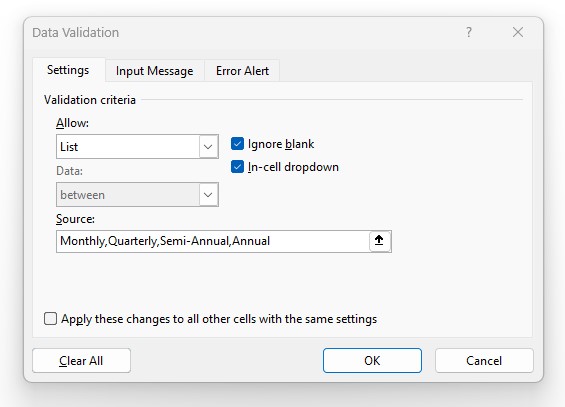
While optional, we’ll create a drop-down list to switch between the payment frequencies using the following steps:

• Step 1 → Select the “Compounding Frequency” Cell (E8)
• Step 2 → Click “Alt + A + V + V” to Open the Data Validation Settings Box
• Step 3 → Pick “List” in the Criteria Section
• Step 4 → Enter “Monthly”, “Quarterly”, “Semi-Annual”, or “Annual” into the “Source” line

In the cell below our drop-down list cell, we’ll enter a formula with a string of “IF” statements to return the figure that corresponds to our active selection.

In effect, if we set our active cell to “Monthly”, our annual interest rate (6.00%) will be divided by 4 while the number of periods (2 Years) is multiplied by 4.

• Monthly Interest Rate = 0.50%
• Number of Periods (nper) = 24 Periods

3. “fv” and “type” Optional Arguments

The “fv” and “type” are the remaining two arguments, both of which we’ll omit here for the following reasons:

• ”fv” → Our assumption for the future value will be left blank as we anticipate the consumer to fulfill all obligations related to the debt and not default, so the value of the loan at maturity should be zero.
• “type” → The timing of the payments was stated earlier as being due at the end of each month, meaning that we can omit it since the default setting in Excel is already set to the end of the period.

4. Excel PPMT Calculation Example

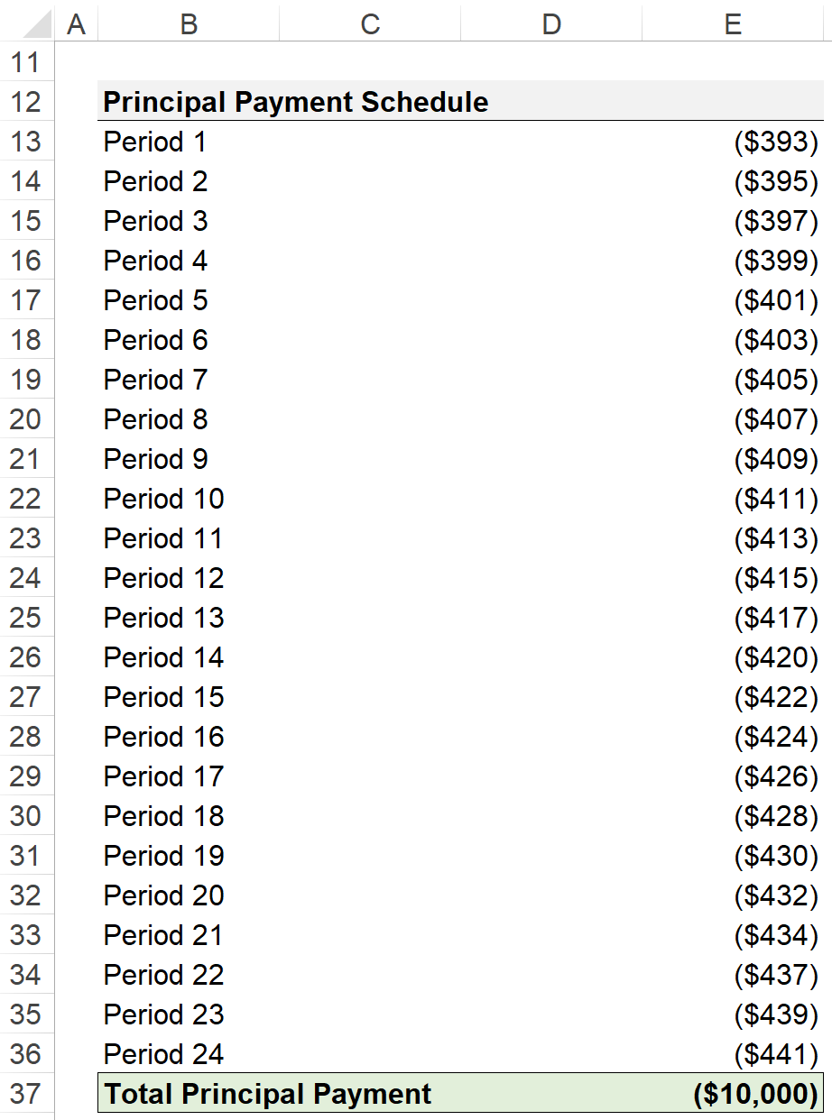
Given the assumptions from the prior steps, we now have the necessary inputs to build our two-year principal payment schedule.

The PPMT formula in Excel for Period 1 is the following:

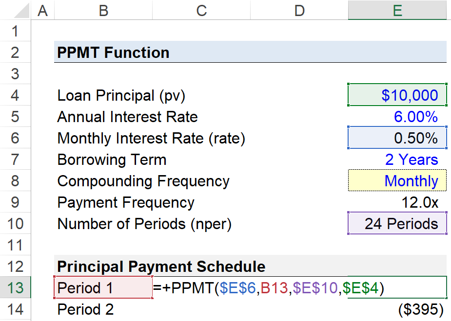
All the arguments, aside from the “per” input, are absolute cell references (F4). The interest rate (”rate”), number of periods (”nper”) and present value (”pv”) are all fixed values that should be kept constant.

Once Period 1 is complete, we can copy-paste the formula down our table (or drag it down) until we reach 24 periods.

5. Principal Payment Schedule Table (=PPMT)

In the final step, we’ll calculate the sum of all principal payments from Period 1 to Period 24.

The total principal payment is ($10,000), confirming our calculation is correct, since the principal value of the loan at issuance was also $10,000.

Turbo-charge your time in Excel

Used at top investment banks, Wall Street Prep’s Excel Crash Course will turn you into an advanced Power User and set you apart from your peers.

Learn More