IPMT Function

How to Use IPMT Function in Excel?

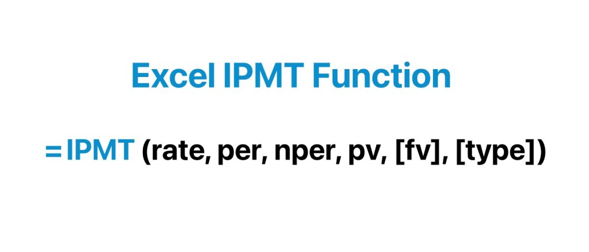
The Excel “IPMT” function calculates the periodic interest payments owed to a lender by a borrower on a loan, such as a mortgage or car loan.

Upon committing to a loan, the borrower is required to pay interest periodically to the lender, as well as repay the original loan principal by the end of the borrowing term.

• Borrower (Debtor) ➝ The interest rate reflects the cost of financing to the borrower, which directly impacts the size of the interest payment (i.e. “cash outflow”)
• Lender (Creditor) ➝ The interest rate reflects the expected return given the risk profile of the borrower, with interest being one of the sources of returns to the lender (i.e. “cash inflow”).

The interest portion of a loan payment can be calculated manually by multiplying the period’s interest rate by the loan principal, which tends to be the norm in financial models.

But the Excel IPMT function was created with that specific purpose in mind, i.e. to calculate the periodic interest owed.

The amount owed in each period is a function of the fixed interest rate and the number of periods that have passed since the date of issuance.

Closer to maturity, the value of the interest payments decline in value alongside the amortizing loan principal balance.

But while the interest paid in each period is based on the outstanding principal balance, the interest payments themselves do NOT reduce the principal.

Real Estate Interview Guide | File Download Form

You’re logged in! Form submission not required. Access your file below.

Download File

Excel IPMT vs. PMT Function: What is the Difference?

The PMT function in Excel calculates the periodic payment on a loan. For example, the monthly mortgage payments a borrower owes.

In contrast, the IPMT calculates only the interest owed; hence the “I” in front.

• IPMT Function ➝ Interest
• PMT Function ➝ Principal + Interest

IPMT function is thereby a part of the PMT function, but the former calculates only the interest component, whereas the latter calculates the entire payment inclusive of both the principal repayment and interest.

Under either calculation, however, there can be other fees and costs incurred, such as taxes, that could affect the yield earned by the lender.

Excel IPMT Function Formula

The formula for using the IPMT function in Excel is as follows.

The inputs with brackets around them—“fv” and “type”—are optional and can be omitted, i.e. either left blank or a zero can be entered.

Since the interest payment is an “outflow” of cash from the perspective of the borrower, the calculated payment will be negative.

For our calculation of the interest payment to be accurate, we must be consistent with our units.

For a quick example, let’s say a borrower took out a 4-year loan with an annual interest rate of 9.0% paid on a monthly basis. In this case, the adjusted monthly interest rate is 0.75%.

• Monthly Interest Rate (rate) = 9.0% ÷ 12 = 0.75%

In addition, the number of periods must be converted appropriately to months by multiplying the borrowing term stated in years by the frequency of payments.

• Number of Periods (nper) = 4 × 12 = 48 Periods

IPMT Excel Function Syntax

The table below describes the syntax of the Excel IPMT function in more detail.

IPMT Function Calculator – Excel Template

We’ll now move on to a modeling exercise, which you can access by filling out the form below.

Excel Template

You’re logged in! Form submission not required. Access your file below.

Download File

1. Interest on Loan Exercise Assumptions

Suppose a consumer has taken out a $200k loan to finance the purchase of an office space.

The loan is priced at an annual interest rate of 6.00% per annum, with payments made on a monthly basis at the end of each month.

• Loan Principal (pv) = $200,000
• Annual Interest Rate (%) = 6.00%
• Borrowing Term = 10 Years
• Compounding Frequency = Monthly (12x)

Because our units are not consistent with one another, the next step is to convert the annual interest rate to a monthly interest rate and convert our borrowing term into a monthly figure.

• Monthly Interest Rate (rate) = 6.00% ÷ 12 = 0.50%
• Number of Periods (nper) = 10 Years × 12 = 120 Periods

2. Frequency of Payments (Create Dropdown List)

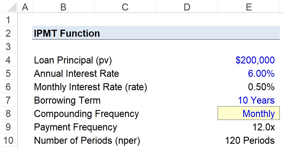
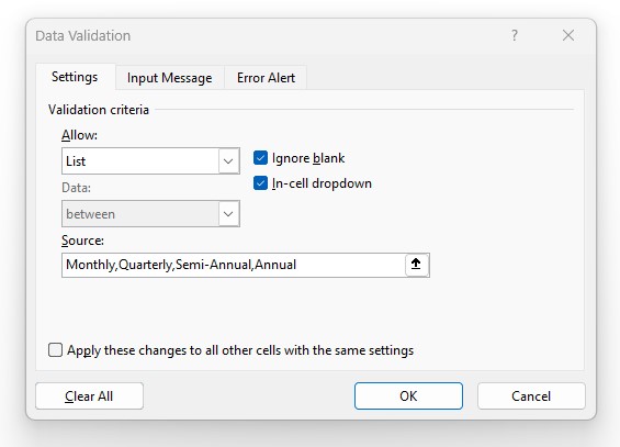
As an optional next step, we’ll create a drop-down list to toggle between the frequency of payments using the following steps:

• Step 1 ➝ Select the “Compounding Frequency” Cell (E8)
• Step 2 ➝ “Alt + A + V + V” Opens Data Validation Box
• Step 3 ➝ Pick “List” in the Criteria
• Step 4 ➝ Enter “Monthly”, “Quarterly”, “Semi-Annual”, or “Annual” into the “Source” line

In Cell E9, we’ll create a formula with a string of “IF” statements to output the corresponding figure we selected in the list.

The remaining two arguments are the “fv” and “type”.

1. Future Value ➝ For “fv”, the input will be kept blank because we’ll assume the loan was fully repaid by the end of the term (i.e. the borrower did not default).
2. Type ➝ The other assumption, “type”, refers to the timing of the payments, which we’ll omit to assume the payments come due at the end of each month.

3. Calculate Interest Payment Using IPMT Excel Function

In the final part of our Excel tutorial, we’ll build our interest payment schedule using the assumptions from the prior steps.

The IPMT formula in Excel we’ll use to calculate the interest each period is as follows.

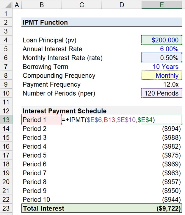
Except for the period column (e.g. B13), the other cells must be anchored by clicking F4.

In conclusion, once our inputs have been entered into the “IPMT” function in Excel, the total interest paid over the ten-year loan comes out to $9,722. The total interest owed on a monthly basis can be seen in our completed interest payment schedule build.

Turbo-charge your time in Excel

Used at top investment banks, Wall Street Prep’s Excel Crash Course will turn you into an advanced Power User and set you apart from your peers.

Learn More