What is SUMIFS Function in Excel?
The SUMIFS Function in Excel returns the sum of the values in a selected cell range that meet a specified set of criteria consisting of multiple conditions.

The SUMIFS Function in Excel returns the sum of the values in a selected cell range that meet a specified set of criteria consisting of multiple conditions.
The Excel SUMIFS function is a built-in feature that adds the value of cells within a range based on a given set of conditions.
The specified criteria consist of logical conditions containing numeric values, dates, or text.
Given those conditions, the SUMIFS function determines which specific cells within the selected range meet the set of conditions using a “TRUE” or “FALSE” logic.
If the user-specified criteria are met, the cell is included in the calculation of determining the sum; otherwise, it is ignored.
For example, one use-case of the SUMIFS function would be to calculate the total amount of revenue contributed by a customer that is located in a certain state. By segmenting customers by states and understanding the concentration, company management can better grasp where their product is most receptive geographically and in which specific areas their current strategy might need improvements.
Simply put, the SUMIFS function is an extension of the SUMIF function, with more capabilities.
In particular, the SUMIFS function in Excel provides the user with the option to select multiple criteria.
While the two functions are near identical with respect to the user’s intent—i.e. to calculate the sum of values in cells that meet a provided criterion—the SUMIFS function is not constrained to only one condition like SUMIF.
Thus, SUMIFS is a more practical function if the task at hand involves a criterion with multiple conditions, rather than only one.
The Excel SUMIFS function formula is as follows.
The brackets around the “sum_range2” and “criteria2” input signify that after the first range and criteria pair, the rest are optional and can be omitted (i.e. left blank).
SUMIFS function can support logical operators and wildcards in the criterion.
In order for the function to work as intended, the proper syntax must be used.
Generally, most operators must be enclosed in double quotes (””) using the proper syntax.
There are exceptions, however, such as purely numeric values or binary conditions.
| Criterion | Description |
|---|---|
| = |
|
| <> |
|
| > |
|
| < |
|
| >= |
|
| <= |
|
| “” |
|
| “<>” |
|
The use of wildcard characters refer to the criterion containing question marks, asterisks, and tildes — the chart below describes each briefly.
| Wildcards | Description |
|---|---|
| ? |
|
| * |
|
| ~ |
|
We’ll now move on to a modeling exercise, which you can access by filling out the form below.


Suppose we’re tasked with segmenting a company’s annual revenue in the trailing twelve months based on two conditions.
The company generated a total of $8 million in revenue with ten customers.
The data set below contains the revenue per customer, customer category, and the state in which the customer is located.
| Customer | Category | State | Revenue |
|---|---|---|---|
| A | Large Enterprise | Pennsylvania | $2,000,000 |
| B | SME | Texas | 700,000 |
| C | SME | Florida | 400,000 |
| D | Large Enterprise | Massachusetts | 2,800,000 |
| E | Large Enterprise | New York | 2,500,000 |
| F | SME | Texas | 400,000 |
| G | Large Enterprise | New York | 2,700,000 |
| H | SME | Texas | 500,000 |
| I | SME | Florida | 400,000 |
| J | Large Enterprise | Massachusetts | 2,600,000 |
| Total Revenue | $15,000,000 |
Using the SUMIFS function, the first range we select is the “Category” column, followed by the customer type criteria. Here, we’ve entered the text in a separate section, so we can link to it directly.
The second range we’ll select is the “State” column, along with the cell reference to the state criteria.
For example, the SUMIFS formula we’ll enter into Excel for the “Large Enterprise” and “New York” pair is as follows.
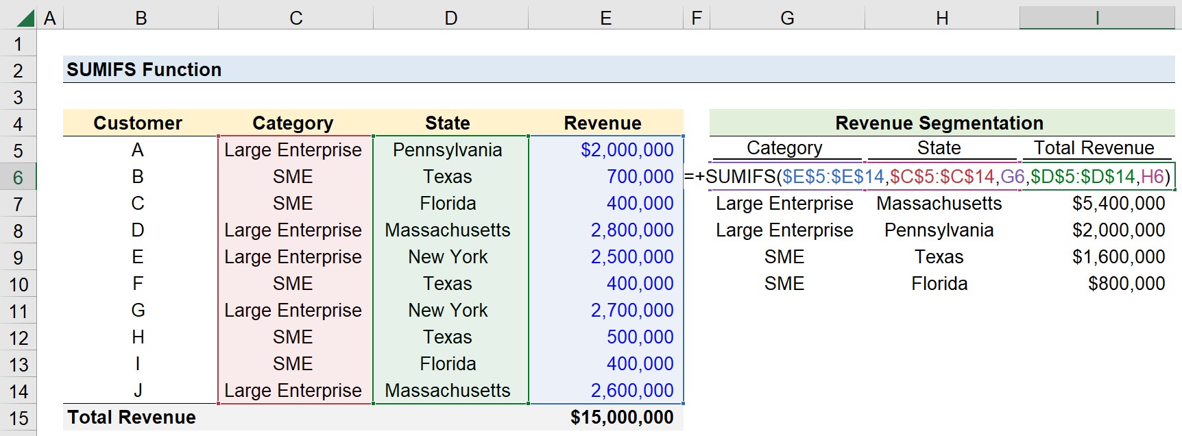
Since we’ll repeat this process for all other pairs, we’ll anchor the range selections by clicking F4 to format it as an absolute reference.
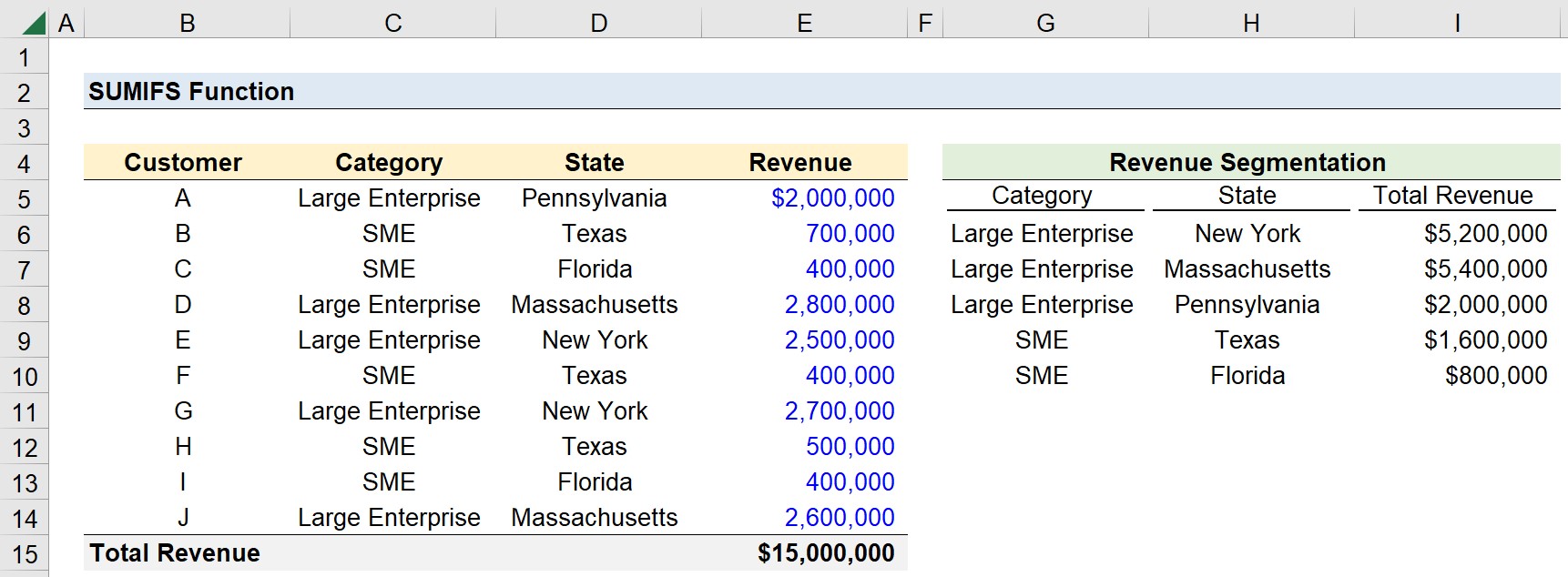
Once done, we arrive at the following revenue distribution data points:



No comments yet.