RATE Function

How to Use RATE Function in Excel?

The usage of the RATE function in Excel is most common for calculating the interest rate on a debt instrument, such as a loan or bond.

The RATE function can also be used to measure the annualized return on an investment or financial metric like revenue – which is termed the compound annual growth rate (CAGR).

The series of cash flows can be either an annuity or lump sum.

• Annuity → A series of payments issued or received in equal installments across time.
• Lump Sum → A single payment is issued or received on a particular date – i.e. paid entirely at once – rather than in a series of payments over time.

Real Estate Interview Guide | File Download Form

You’re logged in! Form submission not required. Access your file below.

Download File

Excel RATE Function Formula

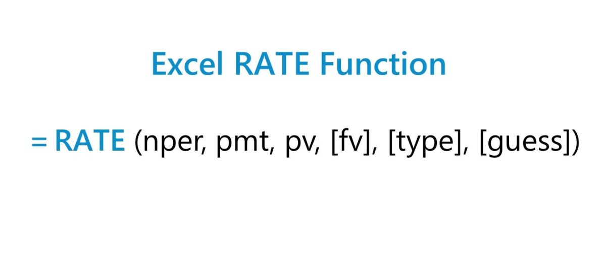
The formula for using the RATE function in Excel is as follows.

The brackets in the latter three inputs of the equation denote that those are optional inputs and can be left blank (i.e. omitted).

RATE Excel Function Syntax

The table below describes the syntax of the Excel RATE function in more detail.

* The “pmt” field could be left omitted, but only if the “fv” – an otherwise optional input – is not

RATE Function Calculator – Excel Model Template

We’ll now move on to a modeling exercise, which you can access by filling out the form below.

You’re logged in! Form submission not required. Access your file below.

Download File

Part 1. Annual Interest Rate on Bond Calculation Example

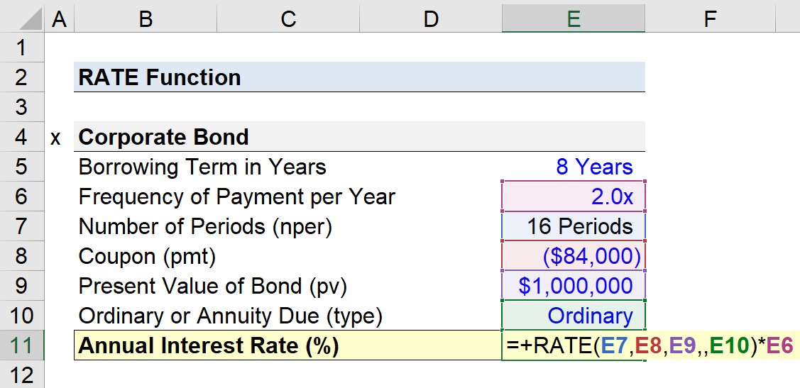
Suppose we’re tasked with calculating the annual interest rate on a $1 million corporate bond issuance.

The financing arrangement is structured as a semi-annual bond, where the coupon (i.e. the interest payment paid semi-annually) is $84k.

• Face Value of Bond (pv) = $1 million
• Semi-Annual Coupon (pmt) = –$84k

The semi-annual corporate bond was issued with a borrowing term of 8 years, so the total number of payment periods comes out to 16.

• Borrowing Term = 8 Years
• Frequency of Payment per Year = 2.0x
• Number of Periods = 8 Years × 2 = 16 Payment Periods

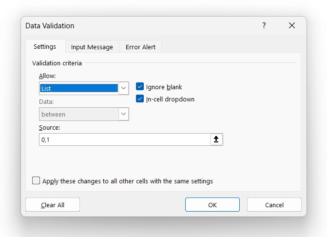
The next optional assumption is the annuity type, where we’ll use the “Data Validation” tool to create a drop-down list to pick between either “0” or “1”.

If “0” is selected, the default setting – an ordinary annuity is assumed. Otherwise, if “1” is selected, the assumption adjusts to an annuity due (and formats the cells accordingly).

While we could technically hard-code "0" or "1" into our Excel formula, creating a drop-down list is not too time-consuming and can reduce the chance of mistakes in the "type" argument.

• Step 1 → Select the “type” Cell (E10)
• Step 2 → Data Validation Keyboard Shortcut: “Alt + A + V + V”
• Step 3 → Pick “List” in the Criteria
• Step 4 → Enter “0,1” into the “Source” line

Once complete, we have all the necessary inputs to calculate the interest rate.

However, the resulting interest rate must then be annualized by multiplying it by the payment frequency.

Since the corporate bond was stated earlier as a semi-annual bond, the adjustment to convert the calculated rate into an annual interest rate is to multiply it by 2.

• Monthly → 12x
• Quarterly → 4x
• Semi-Annual → 2x

Given our set of assumptions, our formula in Excel is as follows.

• Ordinary Annuity → The implied annual interest rate, assuming the payments are received at the end of each period, is 7.4%.
• Annuity Due → In contrast, if we switch our annuity type selection to annuity due, the implied annual interest rate increases to 8.6%.

The intuition is that payments received earlier – as in the case of an annuity due – are worth more because of the time value of money (TVM).

The earlier that cash flows are received, the sooner they can be reinvested, resulting in a greater upside potential in terms of achieving higher returns (and vice versa for cash flows received later).

Part 2. Calculate CAGR Using RATE Function in Excel

In the next section of our exercise, we’ll calculate the compound annual growth rate (CAGR) of a company’s revenue using the Excel RATE function.

In Year 0, our company’s revenue was $100 million, which increased to $125 million by the end of Year 5. The inputs to calculate the five-year CAGR are the following:

• Number of Periods (nper) = 5 Years
• Present Value (pv) = $100 million
• Future Value (fv) = $125 million

The “pmt” field is optional and can be omitted here (i.e. either enter “0” or ",,") because of the fact that we already have the future value ("fv").

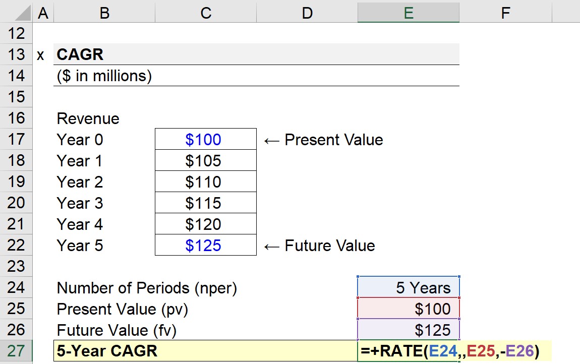
In order for the RATE function to work properly, a negative sign (–) must be placed in front of either the present value or future value.

The implied 5-year CAGR of our hypothetical company’s revenue comes out to 4.6%.

Turbo-charge your time in Excel

Used at top investment banks, Wall Street Prep’s Excel Crash Course will turn you into an advanced Power User and set you apart from your peers.

Learn More