PMT Function

How to Use PMT Function in Excel?

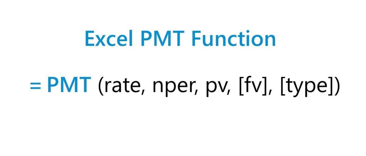
The Excel “PMT” function is used to determine the payments owed to a lender by a borrower on a financial obligation, such as a loan or bond.

The payment owed is derived from a constant interest rate, the number of periods (i.e. loan term), and the value of the original loan principal.

The three variables are assumed to remain fixed across the entirety of the borrowing term.

Note that while the PMT function factors in the original loan principal and interest payments—the two sources of returns to the lender—there can be fees or taxes on the side that impact the lender's "actual" yield.

• Borrower → Because the payment represents an “outflow” of cash from the perspective of the borrower, the resulting payment value will be a negative figure.
• Lender → If wanting to determine the “inflow” of cash received from the viewpoint of the lender, a negative sign can simply be placed in front of the “PMT” equation (to result in a positive figure).

Real Estate Interview Guide | File Download Form

You’re logged in! Form submission not required. Access your file below.

Download File

Excel PMT Function Formula

The formula for using the PMT function in Excel is as follows.

The first three inputs in the formula are required, while the latter two are optional and can be omitted. (Hence, the brackets around “fv” and “type” in the equation.)

In order for the implied payment to be accurate, consistency in the units used (i.e. days, months, or years) is essential.

For instance, if a borrower has taken out a twenty-year loan with an annual interest rate of 5.0% paid on a quarterly basis, then the monthly interest rate is 1.25%.

• Quarterly Interest Rate (rate) = 5.0% ÷ 4 = 1.25%

The number of periods must also be adjusted by multiplying the borrowing term in years (20 years) by the frequency of payments (quarters) per year (4x).

• Number of Periods (nper) = 20 × 4 = 80 Periods (i.e. quarters)

PMT Excel Function Syntax

The table below describes the syntax of the Excel PMT function in more detail.

PMT Function Calculator – Excel Template

We’ll now move on to a modeling exercise, which you can access by filling out the form below.

Excel Template

You’re logged in! Form submission not required. Access your file below.

Download File

Excel PMT Mortgage Loan Payment Calculation Example

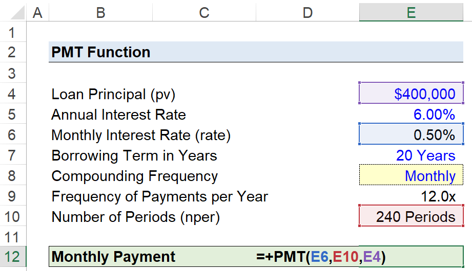
Suppose a consumer has taken out a $400,000 mortgage loan to finance the purchase of a house.

The mortgage loan has an annual interest rate of 6.00% per annum, with payments made on a monthly basis at the end of each month.

• Loan Principal (pv) = $400,000
• Annual Interest Rate (%) = 6.00%
• Borrowing Term in Years = 20 Years
• Compounding Frequency = Monthly (12x)

Since all the necessary assumptions have been provided, the next step is to convert our annual interest rate to a monthly interest rate by dividing it by 12.

• Monthly Interest Rate (rate) = 6.00% ÷ 12 = 0.50%

In order to add the option to switch the compounding frequency, we’ll create a drop-down list to pick the compounding frequency using the following steps:

• Step 1 → Select the “type” Cell (E8)
• Step 2 → “Alt + A + V + V” Opens Data Validation Box
• Step 3 → Pick “List” in the Criteria
• Step 4 → Enter “Monthly”, “Quarterly”, “Semi-Annual”, or “Annual” into the “Source” line

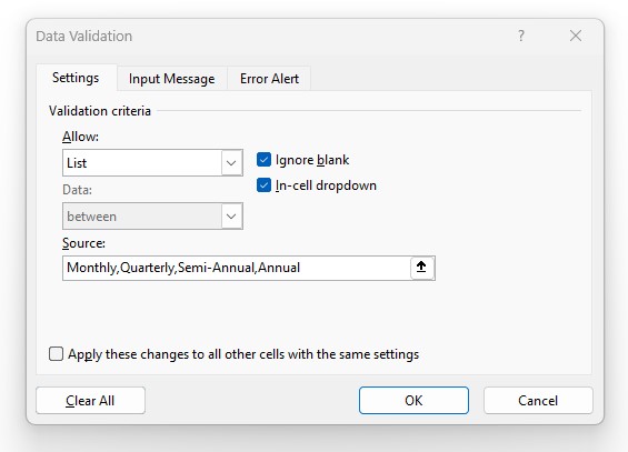
The cell below it will then use an “IF” statement to output the corresponding figure.

While not necessary, per se, the additional step above can help reduce the chance of an error and ensure the correct adjustments are made to the “rate” and “nper” values.

The other adjustment is to the number of periods, in which we’ll multiply the borrowing term in years by the compounding frequency, which comes out to 240 periods.

• Number of Periods (nper) = 20 Years × 12 = 240 Periods

The "fv" and "type" argument will be left omitted since we're assuming that the mortgage will be fully paid off by the end of the borrowing term, and earlier we stated that the payments are due at the end of each month, i.e. the default setting in Excel.

The final step is to enter our inputs into the “PMT” function in Excel, which calculates the implied monthly payment on the twenty-year mortgage as $2,866 per month.

Turbo-charge your time in Excel

Used at top investment banks, Wall Street Prep’s Excel Crash Course will turn you into an advanced Power User and set you apart from your peers.

Learn More