Double Declining Balance Method (DDB)

How the Double Declining Balance Depreciation Method Works

The double declining balance method (DDB) describes an approach to accounting for the depreciation of fixed assets where the depreciation expense is greater in the initial years of the asset's assumed useful life.

But before we delve further into the concept of accelerated depreciation, we’ll review some basic accounting terminology.

• Depreciation → In accounting, the concept of depreciation is the act of writing off the carrying value of a fixed asset (PP&E) across its expected useful life assumption, rather than recording the entire incurred capital expenditure (Capex) in one period.
• Useful Life Assumption → The useful life assumption is the implied number of years in which a fixed asset is assumed to provide economic benefits to the company.
• Salvage Value → The residual value of the fixed asset at the end of its useful life – most companies assume this to be zero.

Certain fixed assets are most useful during their initial years and then wane in productivity over time, so the asset’s utility is consumed at a more rapid rate during the earlier phases of its useful life.

The prior statement tends to be true for most fixed assets due to normal “wear and tear” from any consistent, constant usage.

However, one counterargument is that it often takes time for companies to utilize the full capacity of an asset until some time has passed.

In addition, capital expenditures (Capex) consist of not only the new purchase of equipment but also the maintenance of the equipment. Maintenance capex represents spending related to supporting the existing asset base and its ability to continue to function properly, or perhaps even be more productive (e.g. the customization or upgrade of equipment or integration with other items).

How to Calculate Depreciation in DDB Method

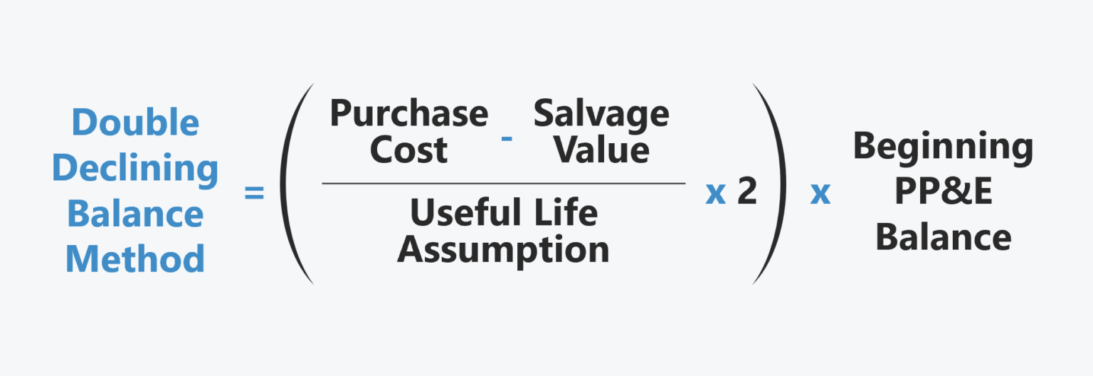
The steps to determine the annual depreciation expense under the double declining method are as follows.

• Step 1 → Calculate the Straight Line Depreciation Expense (Purchase Cost – Salvage Value) ÷ Useful Life Assumption
• Step 2 → Divide the Annual Depreciation Under the Straight Line Method by the Purchase Cost of the Fixed Asset, i.e. the “Straight Line Depreciation Rate”
• Step 3 → Multiply the Straight Line Depreciation Rate by 2x, i.e. the “Double Declining Depreciation Rate”
• Step 4 → Multiply the Beginning Book Value of the Fixed Asset (PP&E) by the Accelerated Rate

Double Declining Balance Method Formula (DDB)

The formula used to calculate annual depreciation expense under the double declining method is as follows.

Double Declining Balance Method vs. Straight Line Depreciation

Even if the double declining method could be more appropriate for a company, i.e. its fixed assets drop off in value drastically over time, the straight-line depreciation method is far more prevalent in practice.

For reporting purposes, accelerated depreciation results in the recognition of a greater depreciation expense in the initial years, which directly causes early-period profit margins to decline.

• Straight Line Depreciation Method → The most common form of depreciation, in which the value of a fixed asset is reduced by an equal value per year, e.g. if an asset with a useful life of 10 years and costs $100 million to purchase, the annual depreciation expense is $10 million each year, assuming a salvage value of zero.
• Double Declining Balance Method → In contrast, accelerated depreciation records greater depreciation expenses in the initial periods post-purchase, but this expense declines over time.

In particular, companies that are publicly traded understand that investors in the market could perceive lower profitability negatively.

Since public companies are incentivized to increase shareholder value (and thus, their share price), it is often in their best interests to recognize depreciation more gradually using the straight-line method.

Of course, the pace at which the depreciation expense is recognized under accelerated depreciation methods declines over time.

However, the management teams of public companies tend to be short-term oriented due to the requirement to report quarterly earnings (10-Q) and uphold their company's share price.

The total depreciation expense recorded across an asset's useful life, at the end of the day, is equivalent under either methodology, yet the straight-line method is more beneficial for increasing short-term profits on a company's financial statements.

Double Declining Balance Method Calculator

We’ll now move on to a modeling exercise, which you can access by filling out the form below.

You’re logged in! Form submission not required. Access your file below.

Download File

1. Fixed Asset Assumptions

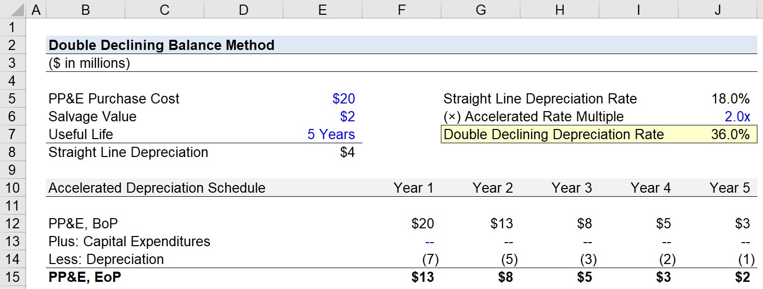
Suppose a company purchased a fixed asset (PP&E) at a cost of $20 million.

Per guidance from management, the PP&E will have a useful life of 5 years and a salvage value of $4 million.

• PP&E Purchase Cost = $20 million
• Salvage Value = $2 million
• Useful Life = 5 Years

2. Straight Line Depreciation Rate Calculation

The next step is to calculate the straight-line depreciation expense, which is equal to the difference between the PP&E purchase price and salvage value (i.e. the depreciable base) divided by the useful life assumption.

• Straight Line Depreciation Expense = ($20 million – $2 million) ÷ 5 Years = $4 million

If the company was using the straight-line depreciation method, the annual depreciation recorded would remain fixed at $4 million each period.

By dividing the $4 million depreciation expense by the purchase cost, the implied depreciation rate is 18.0% per year.

• Straight Line Depreciation Rate = $4 million ÷ $20 million = 18.0%

3. Double Declining Depreciation Rate Calculation

With our straight-line depreciation rate calculated, our next step is to simply multiply that straight-line depreciation rate by 2x to determine the double declining depreciation rate.

• Double Declining Depreciation Rate = 18.0% × 2 = 36.0%

4. Annual Depreciation Expense Calculation (DDB)

We now have the necessary inputs to build our accelerated depreciation schedule.

The beginning of period (BoP) book value of the PP&E for Year 1 is linked to our purchase cost cell, i.e. Year 0.

The depreciation expense recorded under the double declining method is calculated by multiplying the accelerated rate, 36.0% by the beginning PP&E balance in each period.

• Depreciation, Year 1 = $20 million × 36% = ($7 million)
• Depreciation, Year 2 = $13 million × 36% = ($5 million)
• Depreciation, Year 3 = $8 million × 36% = ($3 million)
• Depreciation, Year 4 = $5 million × 36% = ($2 million)

However, note that eventually, we must switch from using the double declining method of depreciation in order for the salvage value assumption to be met. Since we’re multiplying by a fixed rate, there will continuously be some residual value left over, irrespective of how much time passes.

Hence, our calculation of the depreciation expense in Year 5 – the final year of our fixed asset’s useful life – differs from the prior periods.

Instead of multiplying by our fixed rate, we’ll link the end-of-period balance in Year 5 to our salvage value assumption.

The final step before our depreciation schedule under the double declining balance method is complete is to subtract our ending balance from the beginning balance to determine the final period depreciation expense.

• Depreciation, Year 5 = $2 million – $3 million = ($1 million)