Average Cost Method

Average Cost Method for Inventory Accounting

The average cost method, or the “weighted-average method”, is one of the most commonly-used inventory accounting recording policies, only trailing behind FIFO and LIFO.

• FIFO → FIFO is an abbreviation for “First In, First Out.” Under the FIFO approach of inventory accounting, the inventory purchased on an earlier date is recognized first and recorded on the income statement as an expense within the cost of goods sold (COGS) line item.
• LIFO → LIFO is an abbreviation for “Last In, First Out.” Unlike FIFO, LIFO recognizes the most recent purchases of inventories before those purchased earlier, i.e. the most recent inventory purchases are assumed as being the first to be sold and are what are recognized first in COGS.

The average cost method utilizes a weighted average calculation as a compromise between FIFO and LIFO.

The process of calculating the average cost method for inventory recognition is a two-step process.

• Step 1 → The first step is to identify each cost of production incurred in a specified period and the ascribed dollar value.
• Step 2 → In the next step, all of the costs of production are added together and the sum is subsequently divided by the total number of items produced by the company.

With that being said, the weighted average approach implies that each product cost receives equal treatment and that the inventory costs are spread evenly, irrespective of the date of purchase or actual production.

Weighted Average Cost Method vs. FIFO vs. LIFO

The average cost method, relative to FIFO or LIFO, tends to be perceived as a simplistic compromise between the other two inventory accounting methods.

One frequent source of criticism is that the average cost method is improper if the products sold are unique (i.e. a diverse product line), where there is substantial variance in the cost of manufacturing the end product, as well as variance in the selling price.

In practice, the average cost method is most appropriate for companies that sell high-volume products all similarly priced, i.e. the batches of inventories are similar in terms of costs to produce and the sale price.

This limitation of the average cost method is a major reason why widespread adoption of the approach has been slow.

The notable benefit to the weighted average approach is that it is the least time-consuming, yet it can only be used by a particular type of company (i.e. high transaction volume with similarly priced products).

Average Cost Method Formula

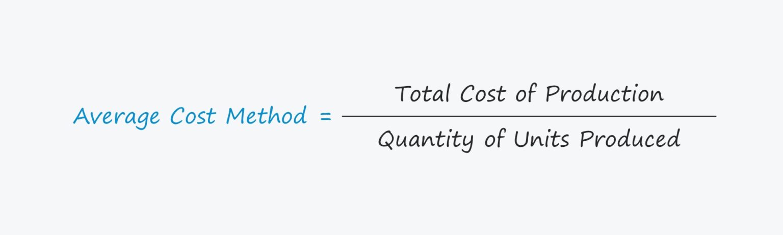
The formula used for the average cost method is as follows.

Average Cost Method Formula

• Average Cost = Total Cost of Production ÷ Quantity of Units Produced

Average Cost Method Calculator – Excel Template

We’ll now move to a modeling exercise, which you can access by filling out the form below.

Excel Template | File Download Form

You’re logged in! Form submission not required. Access your file below.

Download File

Weighted Average Cost Method Example Calculation

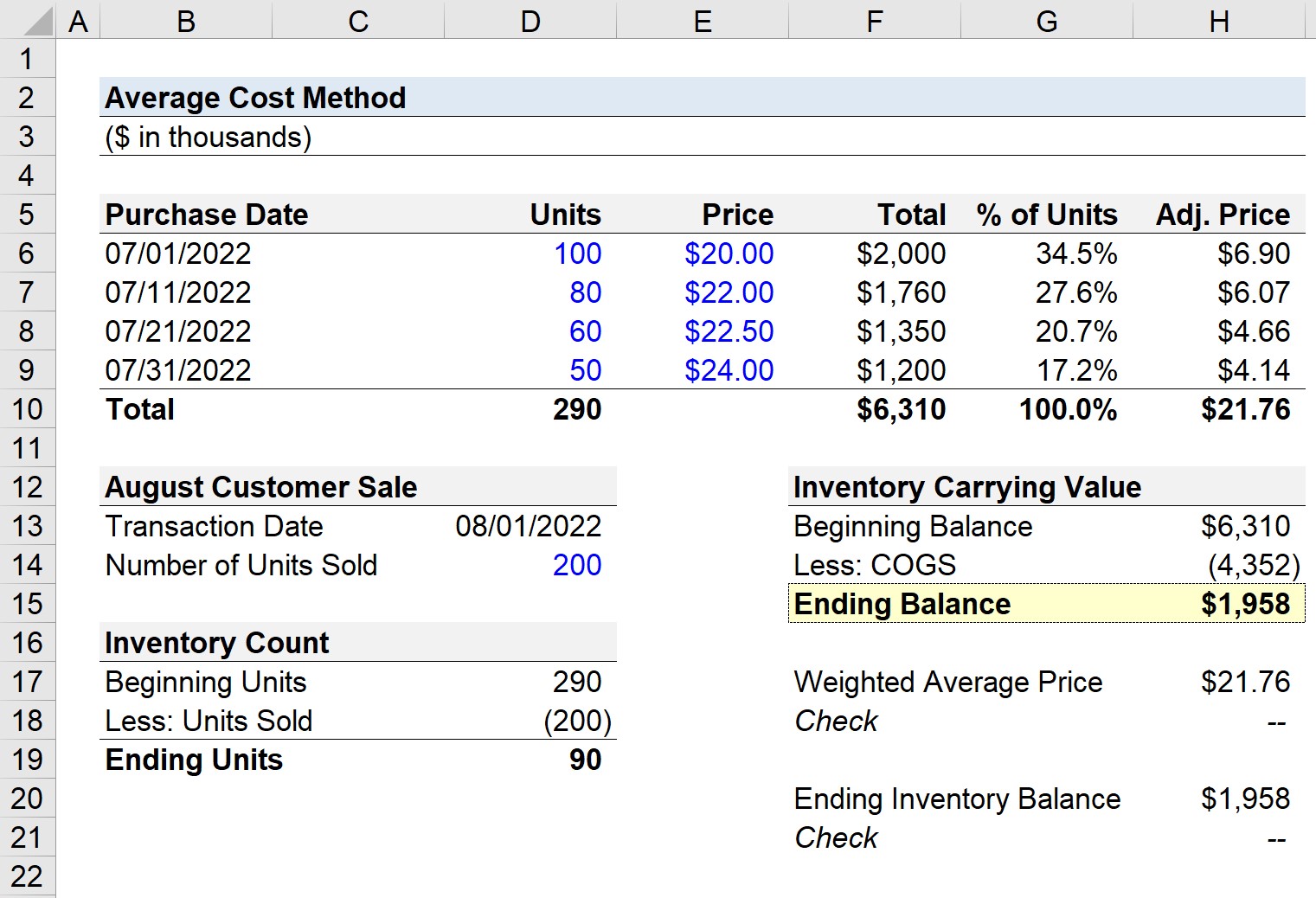
Suppose a company made the following inventory purchases in the month of July 2022.

• Total → The “Total” column refers to the total inventory purchase price for the month of July, which equals the product of the number of units purchased and the corresponding price.
• % of Units → On the right, the “% of Units” is the number of units purchased in the specific batch divided by the total number of units purchased for the month, 290 units.
• Adj. Price → By multiplying the “% of Units” by the stated price, we can calculate the adjusted price of each batch, which factors in all purchases (and the total represents the weighted average price of all purchases).

With our assumptions all set, we’ll now assume that a customer placed a large order of 200 units on August 1, 2022.

In order to calculate the inventory carrying value, we must first determine our inventory count.

The beginning number of units is 290, which represents the total units purchased in July. We’ll subtract 200 units to calculate 90 as the number of ending units.

• Ending Units = 290 – 200 = 90

In the final part of our modeling exercise, we’ll calculate the inventory carrying value, i.e. the value recorded on the balance sheet.

The beginning balance is the weighted average price, $21.76, multiplied by the beginning number of units.

• Beginning Balance = 290 × $21.76 = $6.3 million

Next, the cost of goods sold (COGS) is calculated by multiplying the number of units sold by the weighted average price of $21.76.

• COGS = 200 × $21.76 = $4.4 million

The ending inventory balance is the beginning balance minus COGS, which results in approximately $1.96 million.

• Ending Balance = $6.3 million – $4.4 million = $1.96 million

In closing, we’ll perform two checks to confirm our model is correct.

1. Weighted Average Price: If we divide the total purchase price by the number of units purchased in the month of July, the weighted average price is $21.76, the same as was in our adjusted price column (Column H).
2. Ending Inventory Balance: By multiplying the weighted average price by the number of ending units, we can calculate the ending inventory balance directly, which comes out to $1.96 million (and matches our prior calculation).